R 스터디 10주차
p117~130
회귀분석(Regression Analysis)
두 변수 간의 상관관계를 본다,
제일 단순하게 예측하는 분석 방법
변수 간의 상관 관계가 있고 (x값을 넣었을 때, y값을 도출할 수 있다!(선형적이므로))
변수 간에 선형의 관계가 있고 , 어떤 현상으로부터 관찰 가능한 변수들 간의 인과 관계를 분석하는 기법
hf<-read.csv("http://www.math.uah.edu/stat/data/Galton.csv",
header=TRUE, stringsAsFactors =
FALSE)
head(hf)
str(hf)
str(hf$Gender)
hf$Gender<-factor(hf$Gender)
str(hf$Gender)
hf.son<-subset(hf,
Gender=="M")
head(hf.son)
//필요한 데이터만 고르기(아빠키, 엄마키)
hf.son<-hf.son[c("Father","Mother","Height")]
head(hf.son)
str(hf.son)
//가로 세로 4개의 margin을 줌
par(mar=c(4,4,1,1))
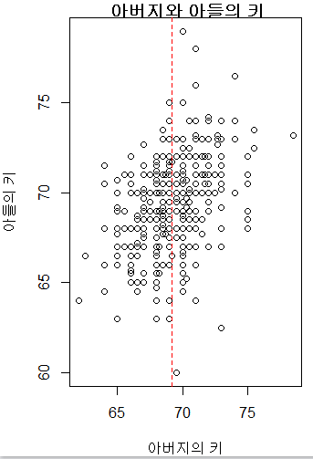
plot(hf.son$Father, hf.son$Height, xlab="아버지의 키",
ylab="아들의 키", main=" 아버지와 아들의 키")

//abline: plot 창에 라인을 추가해라, 아빠 키 평균을 추가해라, col=2(빨간색), lty=2(점선)
abline(v=mean(hf.son$Father),col=2, lty=2)
# col =3 그린
abline(h=mean(hf.son$Height)col=3, lty=5)
# linear model 구하는 공식
# Intercept : y절편

> lm(Height~Father,data=hf.son)

Call:
lm(formula = Height ~ Father, data = hf.son)

Coefficients:
(Intercept)             Father
    38.2589(y절편)       0.4477  (기울기)

# 아들의키  = 38.2589 + 0.4477*x
> summary(hf.son.lm)

Call:
lm(formula = Height ~ Father, data = hf.son)

Residuals:
    Min      1Q  Median      3Q     Max
-9.3774 -1.4968  0.0181  1.6375  9.3987

Coefficients:
            Estimate Std. Error t value Pr(>|t|)
(Intercept) 38.25891    3.38663   11.30   <2e-16 ***
Father       0.44775    0.04894    9.15   <2e-16 ***
---
Signif. codes:  0 ‘***’ 0.001 ‘**’ 0.01 ‘*’ 0.05 ‘.’ 0.1 ‘ ’ 1

Residual standard error: 2.424 on 463 degrees of freedom
Multiple R-squared:  0.1531,    Adjusted R-squared:  0.1513
F-statistic: 83.72 on 1 and 463 DF,  p-value: < 2.2e-16
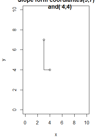
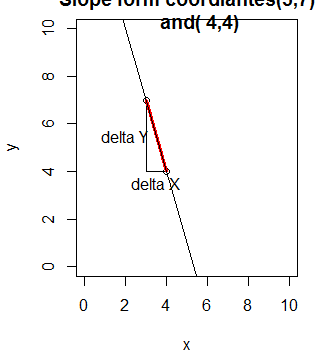
// 직선을 그림으로 나타내기
plot(c(3,4), c(7,4), ylab="y",xlab="x",
main="Slope form coordiantes(3,7)
and( 4,4)", ylim=c(0,10),
xlim=c(0,10))

lines(c(3,3), c(7,4))   //(3,7)에서 하나 찍고(3,7)에서 하나 찍고 이음

lines(c(3,4), c(4,4))

lines(c(3,4), c(4,4))
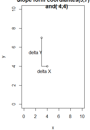
> text(2,5.5, "delta Y")
> text(3.5,3.5, "delta X")
> lines(c(3,4), c(7,4),col="red",lwd=3)
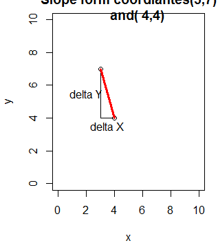
> abline(16,-3)
> plot(c(3,4), c(7,4), ylab="y",xlab="x",      main="Slope form coordiantes(3,7)
+      and( 4,4)", ylim=c(0,10),
+      xlim=c(0,10))
>
> lines(c(3,3), c(7,4))
> lines(c(3,4), c(4,4))
>
> text(2,5.5, "delta Y")
> text(3.5,3.5, "delta X")
>
>
>
> lines(c(3,4), c(7,4),col="red",lwd=3)
>
> abline(16,-3)
> gapdh.qPCR <- read.table(header=TRUE,text='
+ GAPDH RNA_ng A1 A2 A3
+                          std_curve 50 16.5 16.7 16.7
+                          std_curve 10 19.3 19.2 19
+                          std_curve 2 21.7 21.5 21.2
+                          std_curve 0.4 24.5 24.1 23.5
+                          std_curve 0.08 26.7 27 26.5
+                          std_curve 0.016 36.5 36.4 37.2
+                          ')
>
>
> str(gapdh.qPCR)
'data.frame':    6 obs. of  5 variables:
 $ GAPDH : Factor w/ 1 level "std_curve": 1 1 1 1 1 1
 $ RNA_ng: num  50 10 2 0.4 0.08 0.016
 $ A1    : num  16.5 19.3 21.7 24.5 26.7 36.5
 $ A2    : num  16.7 19.2 21.5 24.1 27 36.4
 $ A3    : num  16.7 19 21.2 23.5 26.5 37.2
>
>
> gapdh.qPCR
      GAPDH RNA_ng   A1   A2   A3
1 std_curve 50.000 16.5 16.7 16.7
2 std_curve 10.000 19.3 19.2 19.0
3 std_curve  2.000 21.7 21.5 21.2
4 std_curve  0.400 24.5 24.1 23.5
5 std_curve  0.080 26.7 27.0 26.5
6 std_curve  0.016 36.5 36.4 37.2
>
>
>
> library("reshape2")
Warning message:
package ‘reshape2’ was built under R version 3.3.3
>
>
> gapdh.qPCR <- melt(gapdh.qPCR, id.vars=c("GAPDH",
+                                          "RNA_ng"),
+                    value.name="Ct_Value")
>
> detach("package:reshape2", unload=TRUE)
> library("reshape2", lib.loc="C:/Program Files/R/R-3.3.1/library")
Warning message:
package ‘reshape2’ was built under R version 3.3.3
>
> str(gapdh.qPCR)
'data.frame':    18 obs. of  4 variables:
 $ GAPDH   : Factor w/ 1 level "std_curve": 1 1 1 1 1 1 1 1 1 1 ...
 $ RNA_ng  : num  50 10 2 0.4 0.08 0.016 50 10 2 0.4 ...
 $ variable: Factor w/ 3 levels "A1","A2","A3": 1 1 1 1 1 1 2 2 2 2 ...
 $ Ct_Value: num  16.5 19.3 21.7 24.5 26.7 36.5 16.7 19.2 21.5 24.1 ...
>
> gapdh.qPCR
       GAPDH RNA_ng variable Ct_Value
1  std_curve 50.000       A1     16.5
2  std_curve 10.000       A1     19.3
3  std_curve  2.000       A1     21.7
4  std_curve  0.400       A1     24.5
5  std_curve  0.080       A1     26.7
6  std_curve  0.016       A1     36.5
7  std_curve 50.000       A2     16.7
8  std_curve 10.000       A2     19.2
9  std_curve  2.000       A2     21.5
10 std_curve  0.400       A2     24.1
11 std_curve  0.080       A2     27.0
12 std_curve  0.016       A2     36.4
13 std_curve 50.000       A3     16.7
14 std_curve 10.000       A3     19.0
15 std_curve  2.000       A3     21.2
16 std_curve  0.400       A3     23.5
17 std_curve  0.080       A3     26.5
18 std_curve  0.016       A3     37.2
>
> attach(gapdh.qPCR) // 앞으로 이 데이터 셋을 갖고 놀겠다. 앞으로 쓰는애들은 gapdh.pPCR에 있는 데이터다 !
//dettach()도 있음
>
> names(gapdh.qPCR)
[1] "GAPDH"    "RNA_ng"   "variable" "Ct_Value"
>
> GAPDH
 [1] std_curve std_curve std_curve std_curve std_curve std_curve std_curve
 [8] std_curve std_curve std_curve std_curve std_curve std_curve std_curve
[15] std_curve std_curve std_curve std_curve
Levels: std_curve
>
> RNA_ng
 [1] 50.000 10.000  2.000  0.400  0.080  0.016 50.000 10.000  2.000  0.400  0.080
[12]  0.016 50.000 10.000  2.000  0.400  0.080  0.016
>
> par(mfrow=c(1,2))
>
> plot(RNA_ng, Ct_Value) //로그 함수 처럼 생겼으니, 로그를 씌워주면 선형의 관계로 만들 수 있을 거 같다
>
> plot(log(RNA_ng), Ct_Value)

> model <- lm(Ct_Value ~log(RNA_ng))
> summary(model)

Call:
lm(formula = Ct_Value ~ log(RNA_ng))

Residuals:
    Min      1Q  Median      3Q     Max
-3.0051 -1.7165 -0.1837  1.4992  4.1063

Coefficients:
            Estimate Std. Error t value Pr(>|t|)
(Intercept)  23.8735     0.5382   44.36  < 2e-16
log(RNA_ng)  -2.2297     0.1956  -11.40 4.33e-09

(Intercept) ***
log(RNA_ng) ***R-
---
Signif. codes:
0 ‘***’ 0.001 ‘**’ 0.01 ‘*’ 0.05 ‘.’ 0.1 ‘ ’ 1 //0.001보다 작아요 유의한 모델이에요

Residual standard error: 2.282 on 16 degrees of freedom
Multiple R-squared:  0.8903,    Adjusted R-squared:  0.8835 //R-square가 0.8이면 굉장히 의미있는 모델이다!
F-statistic: 129.9 on 1 and 16 DF,  p-value: 4.328e-09 //0.05보다 작으니 유의한 데이터

> abline(model)
